Machine Learning (ML) is one of the topics in software development that is surrounded by a mystic aura: There is a certain feeling of magic around a piece of code that seems to be able to predict events or recognize complex patterns. This is a reason why ML keeps being confused with Artificial Intelligence.
One of the most common tasks in ML is classification: Creating a model that, after being trained with a dataset, it can label specific examples of data into one or more categories.
In this post, we will use PyTorch -one of the most popular ML tools- to create and train a simple classification model using neural networks (NN).
A warning about PyTorch and Neural networks
For all their power, tools used to create NNs like PyTorch and Tensorflow are not always the best choice for some ML tasks.
Development teams often choose these tools because they are popular and well-known. However, as more experienced ML practitioners will tell you, tasks like classification can more easily be achieved in Python by tools like scikit-learn using models like logistic regression.
Neural networks have a higher complexity than models like linear or logistic regression: They require more fine-tuning of parameters, and often also require more data, training time and computation power.
Having said that, let's review how a simple NN can be constructed for classification; we will revisit this topic in another post using scikit-learn.
A quick primer on Neural networks
Before reading further in this section let me give you a warning: If this is the first time you're reading about neural networks, this part will be complex and hard to fully grasp at first. It is OK if you don't understand what each term in this section means. Feel free to skim through this section and move forward, as the code examples may make things clearer.
The input for a neural network (at both training and prediction time) is a matrix of data of size (r,c), where each row r is a data example and each column c is an attribute. The output depends on the layer structure of the NN, but typically is another matrix of size (r, t), where r is the same number of examples as the input, and t is the number of columns used to represent the result of our model.
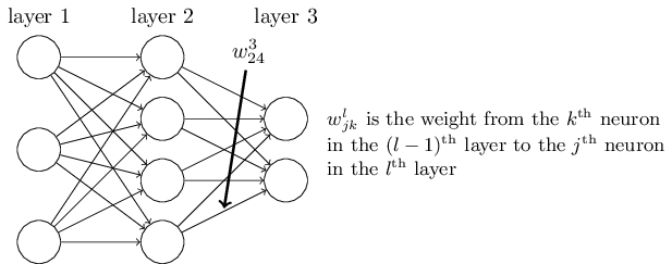
Neural Networks are composed of layers: Each layer transforms the data (e.g. applying a linear transformation by multiplying the matrix of data with a vector of weights that are updated at each step of the training process) and passes it to the next layer for further transformations. The last layer in the network outputs the expected output (in our case, the classification result) for the model.
Individual layers are composed of neurons, where the number of neurons corresponds to the input size of each layer. In the following image we see a network where the first layer (the input layer) has three neurons; so the size of the input layer would be (r=Examples,c=3).

At each training step, we measure the error for the model: How many times the prediction was wrong when compared with a labeled set of test data. The model then uses the error's value and updates the weights to minimize the expected error.
Each layer's weights are updated using a process called backpropagation: The training algorithm calculates the partial derivates of each weight to find the direction in the linear space (remember, weights are vectors) in which we need to update the weight's value for minimizing the expected error in the predictions.
For instance, if the weight needs to increase its value, its partial derivate will point in the opposite direction than the case in which we would need to decrease its value.
For a full in-depth explanation of how Neural Networks and backpropagation work, take a look at the free, online book "Neural Networks and Deep Learning". The following video also provides a great explanation on backpropagation:
The task
For this example, we will address the popular practice problem "Titanic - Machine Learning from disaster" from Kaggle. For those who don't know Kaggle, it is a portal where tons of datasets and data problems can be found. Companies sometimes post their datasets and create contests for people to try to solve specific data problems.
The problem to solve for this dataset is to -given a dataset containing examples of passengers who traveled in the famed ship Titanic, along with an attribute specifying whether they survived the sinking or not- predict whether a specific example of a passenger would have survived.
The model building process
The steps to construct ML models may vary depending on the task at hand. However, most models follow the same pattern:
- Find the data that will use for training
- Load and clean the data
- Encode the data
- Split data into training, test and validation sets
- Define and train the model
- Validate the accuracy of the model
Find the data that will use for training
The data needs to be labeled: A set of multiple examples of the data we plan to use for our predictions, along the label, which in our case is "Survived" -with a value of 1 if the passenger survived, and a value of 0 otherwise. Each column in the data is an attribute, while each row is an instance or example of the data.
Load and clean the data
This is where most of the work of a data engineer is spent. The data will contain multiple undesirable characteristics that would prevent our model from successfully training and predicting:
- Empty attributes. Most of the time, we fill empty attributes with the mean or the mode of the other attributes that do have value. Other times, we might just drop the column or the row.
- Redundant data. For instance, some columns are a direct function of others and don't provide any extra information to the model. We can safely drop these columns.
Encode the data
PyTorch models only accept numeric values as input. We must encode string or categorical columns into numeric values. For this, we have a few options:
- One-hot encoding: Columns that contain categories (e.g. "Sex" contains values like "Male" or "Female") can be converted into numeric values by adding a column for each category, and setting a value of 1 for those columns in that category (and 0 for those that don't).
- Label encoding: Assign direct numeric values to each category (e.g. 1 to "Female" and 2 to "Male"), and replace the string values with their numeric representation. The downside of this approach is that it gives an implicit numeric relationship to the categories: The model will assume that the categories may be ordered when there is no real ordinal relationship in attributes like "Sex".
Split data into training and test sets
Before we start training our model, we must split all our data into three parts: A training set, a test set and a validation set. The majority of the data (e.g. 80%) goes into the training set, and a smaller percentage of the data (let's say 10% and 10%) goes into the test and validation sets. Let me elaborate on why.
At each step of the training process, we want to evaluate our model to see how well the training process is going and make the necessary adjustments. For this, we try to predict a few examples and measure their error.
To avoid overfitting, we take these evaluation examples from a set of data that wasn't used for training (otherwise our model would be "cheating", as it would know the "answer" for those examples). For that, we reserve a part of our dataset and leave it out of the training dataset. To this held out data, we call it test set and the process of using this set during training is called cross-validation.
_Note: To keep things simple we will not use cross-validation for our example, so we will only split our data into training and validation (90%-10%).
Then, once we complete the training of our model, we need to do the last evaluation of the model's performance. For this, we will use the validation set. Keeping the validations set out of the training process will provide a more accurate measure of the model's performance, for the same reason we keep the test set out of the training data.
A great explanation of the importance and process of splitting datasets can be in this post by Cassie Kozyrkov.
Define and train the model
Defining the model is the second most important task in this process.
In the case of NNs, we must define the number and size of each layer in the network, activation layers, and the hyperparameters for the training (batch size, learning rates, number of training iterations and so on). This configuration is what makes NNs more complex to define and train than simpler models like logistic regression.
Validate the accuracy of the model
Finally, we use our trained model to make predictions on our validation data set. We compare the answers given by the model with the actual labels of the validation set, and we calculate the statistical information of how many times the model did a bad prediction. Some measures of this performance are accuracy, precision, recall and F1. Here's a post about each of these measurements and how they reflect different parts of a model's performance.
The code
You can find all the code used in this example in this Google Collab notebook. This whole example is written in Python, so we will use Python libraries for ML.
In this example, we will use:
- Pandas to load and manipulate our dataset.
- numpy for matrix and vector operations.
- scikit-learn for splitting our dataset
- PyTorch for building the NN.
import numpy as np
import pandas as pd
from sklearn.model_selection import train_test_split
Read the data from the CVS files
We download the train.csv dataset from Kaggle and put it in the same directory as our Python code.
The following is a table with the description of each attribute in the data:
| Variable | Definition | Key |
|---|---|---|
| survival | Survival | 0 = No 1 = Yes |
| pclass | Ticket class | 1 = 1st 2 = 2nd 3 = 3rd |
| sex | Sex | |
| Age | Age in years | |
| sibsp | # of siblings / spouses aboard the Titanic | |
| parch | # of parents / children aboard the Titanic | |
| ticket | Ticket number | |
| fare | Passenger fare | |
| cabin | Cabin number | |
| embarked | Port of Embarkation | C = Cherbourg Q = Queenstown S = Southampton |
We then load our data into memory using Pandas:
train = pd.read_csv('train.csv')
We can see some examples of the dataset using Panda's head method:
train.head()
| PassengerId | Survived | Pclass | Name | Sex | Age | SibSp | Parch | Ticket | Fare | Cabin | Embarked | Title | FamilySize | |
|---|---|---|---|---|---|---|---|---|---|---|---|---|---|---|
| 0 | 1 | 0 | 3 | Braund, Mr. Owen Harris | male | 22 | 1 | 0 | A/5 21171 | 7.25 | nan | S | Mr | Couple |
| 1 | 2 | 1 | 1 | Cumings, Mrs. John Bradley (Florence Briggs Thayer) | female | 38 | 1 | 0 | PC 17599 | 71.2833 | C85 | C | Mrs | Couple |
| 2 | 3 | 1 | 3 | Heikkinen, Miss. Laina | female | 26 | 0 | 0 | STON/O2. 3101282 | 7.925 | nan | S | Miss | Single |
| 3 | 4 | 1 | 1 | Futrelle, Mrs. Jacques Heath (Lily May Peel) | female | 35 | 1 | 0 | 113803 | 53.1 | C123 | S | Mrs | Couple |
| 4 | 5 | 0 | 3 | Allen, Mr. William Henry | male | 35 | 0 | 0 | 373450 | 8.05 | nan | S | Mr | Single |
Clean the data
A few transformations are needed:
- Drop columns that don't provide information for the classification. For instance, the ticket number
ticketprovides little to no information to predict if a passenger survived that cannot be found in other attributes in the data. - Fill empty values (e.g. fill empty `age`` values with the median of existing age records)
- Group columns into more meaningful labels:
- E.g. add the values
SibSpandParchinto a single categoryFamilySize. - Transform
FamilySizeinto a category (e.g.single,couple,large).
- E.g. add the values
- Drop redundant columns (e.g.
SibSpandParch, as they have been merged intoFamilySize)
If you imported more than one dataset (like an extra test dataset, or unlabeled data to predict), this cleanup needs to be done for all of them.
Note: Data cleanup is specific to the dataset. You need to understand what your dataset is trying to achieve, which columns have a direct relation with the prediction result, which columns are unnecessary and how to better fill empty values and group categories.
def clean_data(dataset):
  dataset_title = [i.split(',')[1].split('.')[0].strip() for i in dataset['Name']]
  dataset['Title'] = pd.Series(dataset_title)
  dataset['Title'].value_counts()
  dataset['Title'] = dataset['Title'].replace(['Lady', 'the Countess', 'Countess', 'Capt', 'Col', 'Don', 'Dr', 'Major', 'Rev', 'Sir', 'Jonkheer', 'Dona', 'Ms', 'Mme', 'Mlle'], 'Rare')

  dataset['FamilySize'] = dataset['SibSp'] + dataset['Parch'] + 1

  def count_family(x):
    if x < 2:
        return 'Single'
    elif x == 2:
        return 'Couple'
    elif x <= 4:
        return 'InterM'
    else:
        return 'Large'

  dataset['FamilySize'] = dataset['FamilySize'].apply(count_family)
  dataset['Embarked'].fillna(dataset['Embarked'].mode()[0], inplace=True)
  dataset['Age'].fillna(dataset['Age'].median(), inplace=True)
  dataset = dataset.drop(['PassengerId', 'Cabin', 'Name', 'SibSp', 'Parch', 'Ticket'], axis=1)
  return dataset


train_clean = clean_data(train)

print(train_clean)

X = train_clean.iloc[:, 1:]
y = train_clean.iloc[:, 0]

X
We can find some examples of the result of this data cleanup.
| Pclass | Sex | Age | Fare | Embarked | Title | FamilySize | |
|---|---|---|---|---|---|---|---|
| 0 | 3 | male | 22.0 | 7.2500 | S | Mr | Couple |
| 1 | 1 | female | 38.0 | 71.2833 | C | Mrs | Couple |
| 2 | 3 | female | 26.0 | 7.9250 | S | Miss | Single |
| 3 | 1 | female | 35.0 | 53.1000 | S | Mrs | Couple |
| 4 | 3 | male | 35.0 | 8.0500 | S | Mr | Single |
| ... | ... | ... | ... | ... | ... | ... | ... |
| 886 | 2 | male | 27.0 | 13.0000 | S | Rare | Single |
| 887 | 1 | female | 19.0 | 30.0000 | S | Miss | Single |
| 888 | 3 | female | 28.0 | 23.4500 | S | Miss | InterM |
| 889 | 1 | male | 26.0 | 30.0000 | C | Mr | Single |
| 890 | 3 | male | 32.0 | 7.7500 | Q | Mr | Single |
Encode data
PyTorch only accepts numbers for attributes, so we convert all categorical/string data into numbers.
pd.get_dummies gets the values in categorical_columns and creates a
new numeric column for each category in those columns (e.g. the
Sex:{male, female} column is split into two columns: SexMale:
0 and SexFemale: {1, 0} )
Just as with data cleanup, this also needs to be done for unlabeled data for which we will try to get actual predictions out of the trained model
def encode_data(X):
  categorical_columns = ['Pclass','Sex', 'FamilySize', 'Embarked', 'Title']

  X_enc = pd.get_dummies(X, prefix=categorical_columns, columns = categorical_columns, drop_first=True)
  return X_enc

X_enc = encode_data(X)
X_enc.head()
| Age | Fare | Pclass_2 | Pclass_3 | Sex_male | FamilySize_InterM | FamilySize_Large | FamilySize_Single | Embarked_Q | Embarked_S | Title_Miss | Title_Mr | Title_Mrs | Title_Rare | |
|---|---|---|---|---|---|---|---|---|---|---|---|---|---|---|
| 0 | 22.0 | 7.2500 | 0 | 1 | 1 | 0 | 0 | 0 | 0 | 1 | 0 | 1 | 0 | 0 |
| 1 | 38.0 | 71.2833 | 0 | 0 | 0 | 0 | 0 | 0 | 0 | 0 | 0 | 0 | 1 | 0 |
| 2 | 26.0 | 7.9250 | 0 | 1 | 0 | 0 | 0 | 1 | 0 | 1 | 1 | 0 | 0 | 0 |
| 3 | 35.0 | 53.1000 | 0 | 0 | 0 | 0 | 0 | 0 | 0 | 1 | 0 | 0 | 1 | 0 |
| 4 | 35.0 | 8.0500 | 0 | 1 | 1 | 0 | 0 | 1 | 0 | 1 | 0 | 1 | 0 | 0 |
Split test data into train and validation datasets
We split our training data into train and val. During training, the
model will learn using train and we then will use val to measure the
number of times our model predicted correctly or not.
We split 90% for training and 10% of data for validation.
Don't forget to also split the labels y, so they are assigned to the
correct sub-datasets
# split training data into training and test
x_train, x_val, y_train, y_val = train_test_split(X_enc, y, test_size = 0.1)
We confirm that the data has been split in the expected percentages
print(X_enc.shape, x_train.shape, x_val.shape)
(891, 14) (801, 14) (90, 14)
The PyTorch model
This PyTorch model defines a neural network with the following layers:
- Linear transformation with an input of 14 columns (one for each of our data columns, after cleanup and encoding), and output of size 270
- A dropout layer with a chance of %1 of dropping a specific row (for reducing overfitting).
- A ReLu activation layer
- Another linear transformation with an input of 270 (the output of the first linear transformation) and an output of 2 (the probabilities of surviving/not surviving)
Here are some links for resources, if you want to gain more understanding of each of these components:
- https://pytorch.org/docs/stable/generated/torch.nn.Linear.html
- https://pytorch.org/docs/stable/generated/torch.nn.Dropout.html
- https://machinelearningmastery.com/rectified-linear-activation-function-for-deep-learning-neural-networks/
# Pythorch model:

import torch
import torch.nn as nn
import torch.nn.functional as F

class Model(nn.Module):

    def __init__(self):
        super(Net, self).__init__()
        self.fc1 = nn.Linear(14, 270)
        self.fc2 = nn.Linear(270, 2)

    def forward(self, x):
        x = self.fc1(x)
        x = F.dropout(x, p=0.1)
        x = F.relu(x)
        x = self.fc2(x)
        x = torch.sigmoid(x)

        return x

model = Model()
Training parameters
The following are the hyperparameters we will set into our model:
- We train the model in batches of 50 samples to avoid over-fitting.
- We train the model for 50 epochs/iterations, to iteratively train the model.
- We train the model with a learning rate of 0.01
- To calculate the error during training (which will allow the model to update weights through backpropagation), we use the Cross entropy loss function (commonly used for binary classification).
- We use the Adam optimizer for finding the gradients.
Some more information on cross-entropy loss can be found in [this article](https://pytorch.org/docs/stable/generated/torch.nn.CrossEntropyLoss.html https://analyticsindiamag.com/ultimate-guide-to-pytorch-optimizers/).
# Model params:
batch_size = 50
num_epochs = 50
learning_rate = 0.01
batch_no = len(x_train) // batch_size

criterion = nn.CrossEntropyLoss()
optimizer = torch.optim.Adam(net.parameters(), lr=learning_rate)
Train the model
We train the network model. More details in the code comments.
from sklearn.utils import shuffle
from torch.autograd import Variable

# Iterate for the number of epochs
for epoch in range(num_epochs):
    # Print the epoch number every 5 epochs
    if epoch % 5 == 0:
        print('Epoch {}'.format(epoch+1))

    # Shufle the datasets to randomize the data rows that
    # will be added to the batch and avoid training over the same 50 rows
    # at each epoch
    x_train, y_train = shuffle(x_train, y_train)
    # Mini batch learning
    for i in range(batch_no):
        start = i * batch_size
        end = start + batch_size

        # Convert the Pandas dataset into PyTorch variables of the size
        # of the batch
        x_var = Variable(torch.FloatTensor(x_train.values[start:end]))
        y_var = Variable(torch.LongTensor(y_train.values[start:end]))

        # Restart the gradients
        optimizer.zero_grad()

        # Run a training step: Pass the training data to
        # the neural network layers
        ypred_var = model(x_var)

        # Calculate the training loss
        loss =criterion(ypred_var, y_var)

        # update the gradients based on the training loss for the batch
        loss.backward()
        optimizer.step()
Epoch 1
Epoch 6
Epoch 11
Epoch 16
Epoch 21
Epoch 26
Epoch 31
Epoch 36
Epoch 41
Epoch 46
Measure the model's performance
We now predict the labels for our validation set x_val.
The results of the prediction in result = model(test_var) will be a
matrix of where the rows are the predicted values for each validation
row, and the columns are:
- The percentage of probability that the passenger survived
- The percentage of probability that the passenger didn't survive
Both columns should add up to 1 for a given row, and the closer to 1 for each of those columns, the most certain the model is about the result
## convert the Pandas dataframe for the validation data to a PyTorch variable
validation_data = Variable(torch.FloatTensor(x_val.values), requires_grad=True)

## Use "no_grad" to not update the model's gradients, as we are not training
## this model anymore
with torch.no_grad():
    ## get the predicted values
    result = model(validation_data)

## Sample 5 results
result[0:5, :]
tensor([[1.0000e+00, 1.0036e-13],
        [9.9993e-01, 5.8530e-14],
        [1.0000e+00, 1.0000e+00],
        [1.0000e+00, 1.0000e+00],
        [9.9999e-01, 5.0890e-12]])
Since we want a binary classification (survived/didn't survive), we get the result with the highest percentage of confidence (1=survived, otherwise 0) using PyTorch's max function.
values, labels = torch.max(result, 1)
## sample the first 5 results
labels[0:5]
tensor([0, 0, 0, 0, 0])
For measuring the model's performance, we calculate a simple percentage of accuracy:
num_right= the number of rows where the prediction matched the actual value in the validation setall_rows= the total number of rowsaccuracy=num_right/all_rows
num_right = np.sum(labels.data.numpy() == y_val)
all_rows = len(y_val)
print('Accuracy {:.2f}'.format(num_right / all_rows))
Accuracy 0.78
As the number of correctly predicted examples increases, the accuracy will also increase. In theory, a perfect model would achieve an accuracy of 1.0, and the worst classifier -which is smart enough to beat the probability of getting a result right by accident, and always chooses the wrong prediction- would achieve an accuracy of 0.0.
Performance is an extremely subjective concept. An accuracy of 0.78 is really good for this problem, but when we are dealing with problems that have a critical impact on people's lives (medical and finance-related problems), 0.78 may not be good enough for considering a model as performant.
An observation about the accuracy results
The accuracy is based only on the existing examples in the dataset. Once we use it in data outside of this dataset, accuracy may be lower as new data may contain attributes that don't exist in this dataset or may have attributes that indicate a different correlation to the classification result. This is why, the more training data we have, the more accurate our performance measurement will be.
The accuracy will also vary between model training executions, as the training data is split randomly between the training and validation datasets.
Notice that accuracy is a kind-of misleading metric: If the model predicts all data samples as "survived" (which is indicative of an incorrect model), you might still get relatively high accuracy. This is why we use other metrics like the F1 score, and do further analysis on the results with analysis tools like confussion matrices and visual representations of the data.
Another downside of just looking at accuracy leaves out a lot of information that may be critical for evaluating a model. Going back to the example of medical applications: For a model that predicts whether a patient has some sort of disease based on their medical history, the impact of a false negative -predicting false when the patient does have the disease- is considerably higher than those of false positives -predicting a patient may have the disease when they don't-.
A false positive can be corrected by doctors performing more studies on the patient, while false negatives may leave a patient without the treatment they need. Precision and recall are good metrics to know -in addition to accuracy- in this case.
Conclusion
In this post we created and trained a neural network for classification in PyTorch.
The work for building Machine Learning models is 80% data analysis and cleanup, and 20% model configuration and coding. The model's performance will depend completely on the data we use to train it; If the data is not clean (it has multiple empty values or redundant information), the model's performance will suffer.
Neural Networks are a powerful tool for ML tasks, but they also have added complexity that other, more focused, tools. This example could have been solved with logistic regression, with similar performance. The added complexity of NNs can lead to over-complicated models that perform worst than simpler models.
NNs also require some understanding of more complex topics like backpropagation, which can be a roadblock for people starting to work in ML.
Having said that, NNs have the advantage of capturing hidden signals in the dataset that would require extra effort in data engineering to get a good performance in simpler models.

